RStudio Activity, a project that is meant as an introduction into R
We have done a project using R (the coding language) for first time and RStudio, an environment for R. The data that we have collected is about pollutants and some wind properties.
Process and code, DATA SECTION: |
Photography: |
|---|---|
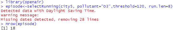
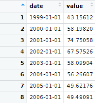
In this section you will see all the data and documents that we will be using to create the graphics. First of all, I had to link R and RStudio to get into the main interface. Next, I had to download three libraries that will be required to do the following steps. This is the code to install the libraries: install.packages (c("tidyverse","openair","dplyr")) Or if It doesn't work: install.packages("tidyverse") install.packages("openair") install.packages("dplyr") Secondly, what we have to do is to download the data that we will be using and organize that code. I download the data from here: Pollutant data and Wind data (these webs are in my native language). The data has to be in the .csv format (you can see It in the properties of the document). POLLUTANTS:Create a new project in RStudio. Here you can see the code, city is the name of the document and what is in brackets is the location of the document:city<-read.csv("C://Users/YOURCOMPUTERNAME/Documents/city.csv") View(city) library(tidyverse) city2<-city1[-c(1,2,4,6:16)] write.csv(city2,"C:\\Users\\YOURCOMPUTERNAME\\Documents\\city2.csv") We delete T 00.00.00.000 and replace the hours h01, etc by 01:00:00 until obtaining the dates in format ISO: We combine date and time together in city4.csv using LibreOffice Calc, RStudio or Visual Code Studio: city4 <- city3 %>% mutate(name=paste0(data, " ", hour)) We create city5 by joining day and time under the name of date. We convert the data format:library(openair) city5PM10 <- subset(city5, pollutant=="PM10") city5PM10$date<-as.POSIXct(city5PM10$date,"%Y-%m-%d %H:%M:%S", tz="Europe/Madrid") View(city5PM10) Care must be taken that the date is not a set of characters (character) but a POSIX, a date. Sorting data with pivot_wider:library(tidyverse) library (openair) city6<-pivot_wider(city5, names_from= pollutant, values_from =value) write.csv(city6,"C:\\Users\\ELMEUNOM\\Documents\\MYCITY\\city6.csv") city6$date<- as.POSIXct(city6$date,format="%Y-%m-%d %H:%M:%S",tz="Europe/Madrid") Daily:daily<-timeAverage(city5PM10,avg.time = "day") View(daily) Yearly:yearly<-timeAverage(city5PM10,avg.time = "year") View(yearly) Yearlyall:yearlyall<-timeAverage(city5,avg.time = "year") View(yearlyall) yearlyall$date<-as.POSIXct(yearlyall$date,"%Y-%m-%d, tz="Europe/Madrid") Episode:episode<-selectRunning(city6, pollutant="O3",threshold=120, run.len=8) nrow(episode) R tells us that the level of 120 micrograms / cubic meter has been exceeded in the average of 8h a total of 95 times. In my case: [1] 18 WIND:wind<-read.csv("C://Users/YOURCOMPUTERNAME/Documents/wind.csv") View(wind) wind1<-wind[-c(1,2,5,7,8)] library(tidyverse) wind2<-pivot_wider(wind1,names_from = CODI_VARIABLE, values_from = VALOR_LECTURA) names(wind2)[names(wind2) == "31"] <- "wd" names(wind2)[names(wind2) == "30"] <- "ws" names(wind2)[names(wind2) == "DATA_LECTURA"] <- "date" write.csv(wind2,"C:\\Users\\YOURCOMPUTERNAME\\Documents\\wind2.csv") We eliminate the X column in libreoffice, It's created wind3. library(openair) wind4<-timeAverage(wind3, time.avg="hour") |
|
You can right click on the graphics to download them or to see them bigger ↓
Process and code, GRAPHIC SECTION: |
Photography: |
|---|---|
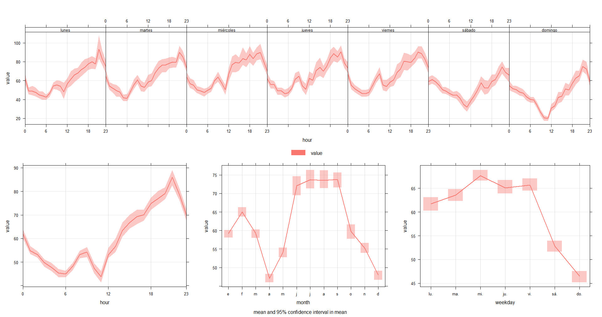
Time Variation:timeVariation(city5PM10, pollutant="value") |
 |
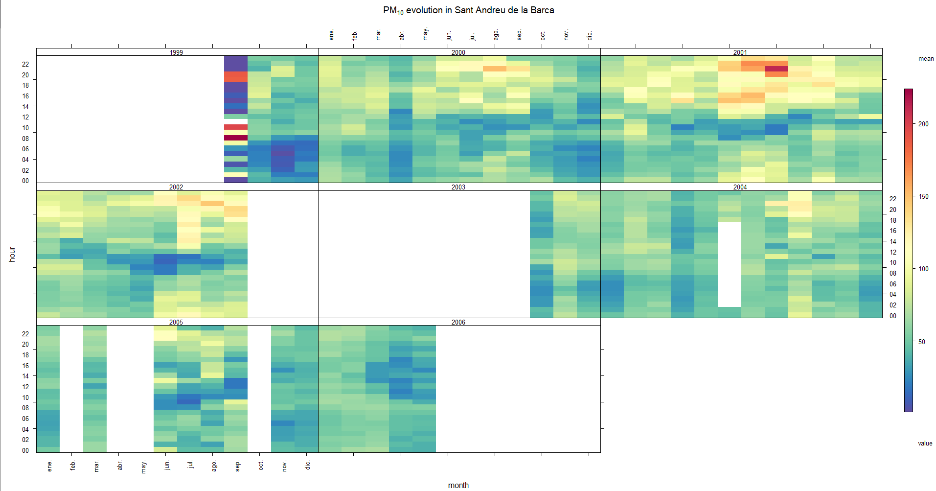
Trend Level:trendLevel(city5PM10, pollutant = "value", main="Hydrogen sulfide evolution in MYCITYNAME") |
 |
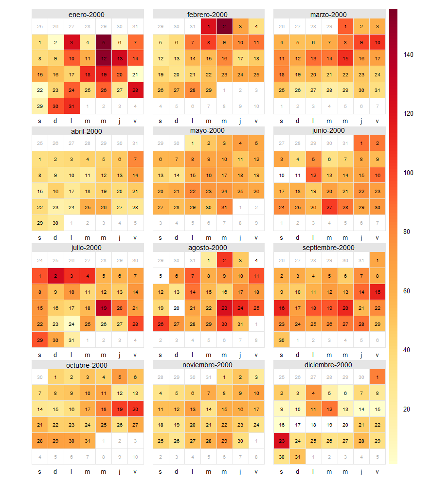
Calendar Plot:calendarPlot(city%NO2, pollutant="value", year="2020") |
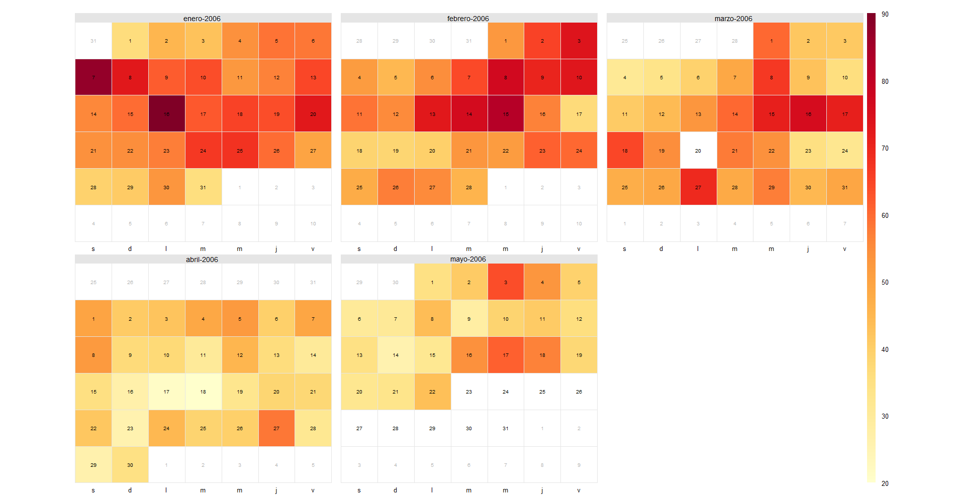 |
Calendar Plot 2:calendarPlot(city%PM10, pollutant="value", year="2020") |
 |
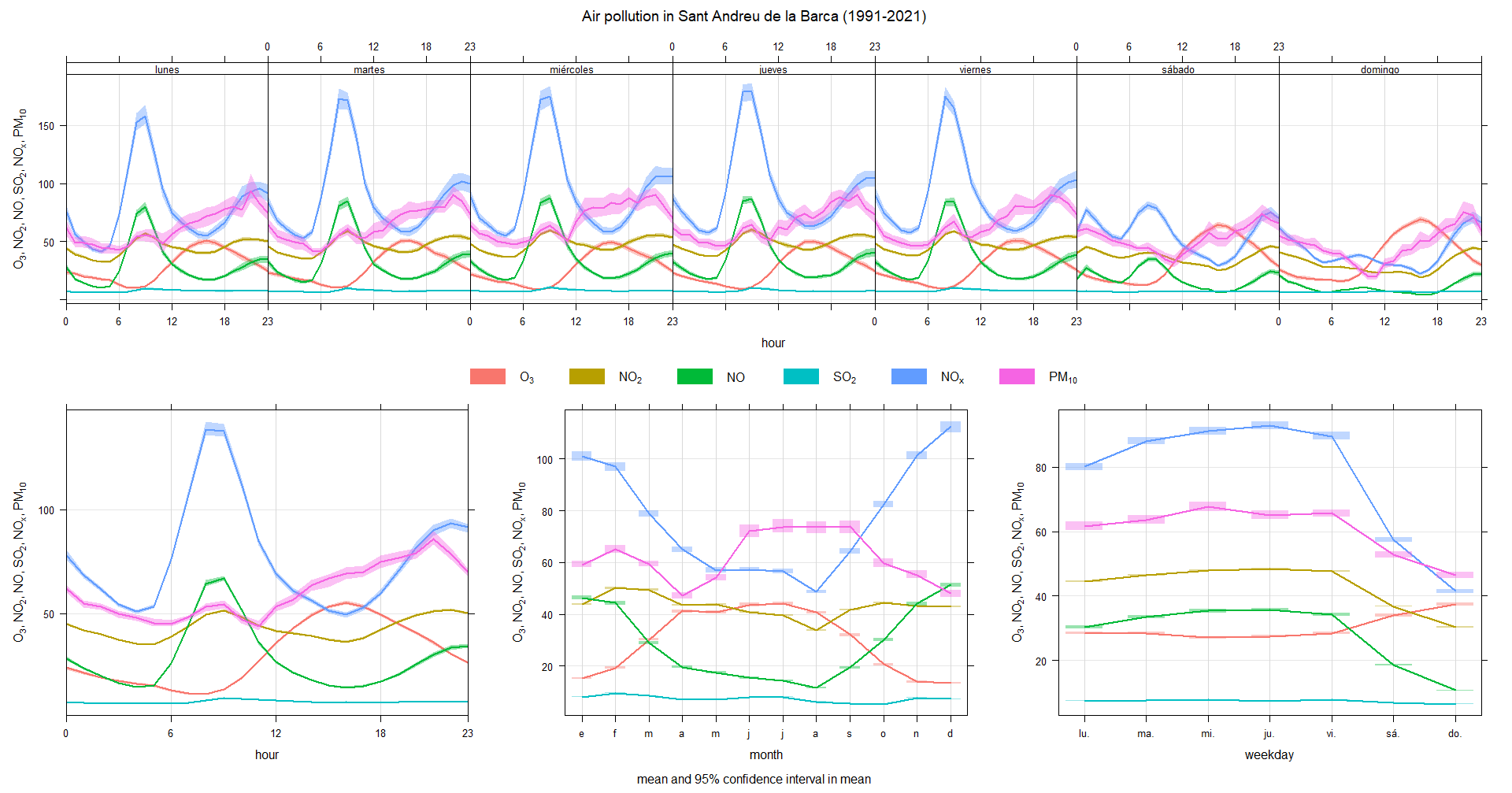
Temporary variation of pollutants 1991-2021:timeVariation(city6, pollutant=c("O3","NO2","H2S","NO","HCNM","CO","SO2","HCT", "NOX","PM10"), main="Air pollution in MYCITYNAME (1991-2021)") |
 |
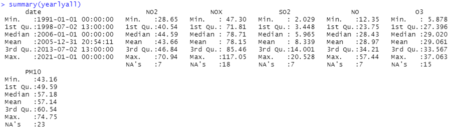
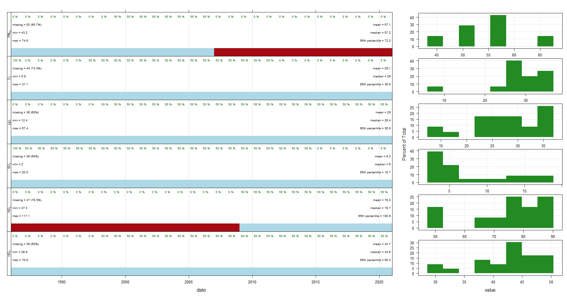
Summary Plot:summaryPlot(yearlyall) |
 |
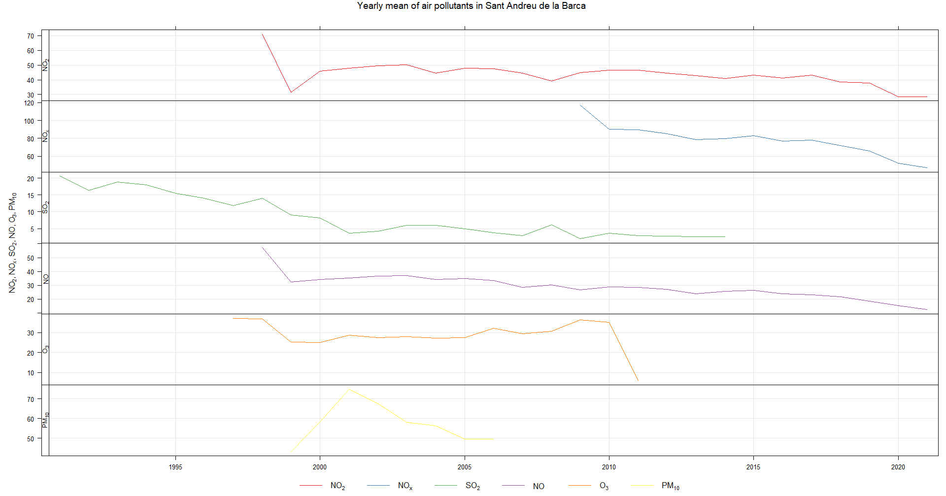
Time Plot:timePlot(selectByDate(yearlyall), pollutant = c("NO2", "NOX", "SO2", "NO", "O3", "PM10"), y.relation = "free", main="Yearly mean of air pollutants in Sant Andreu de la Barca") |
 |
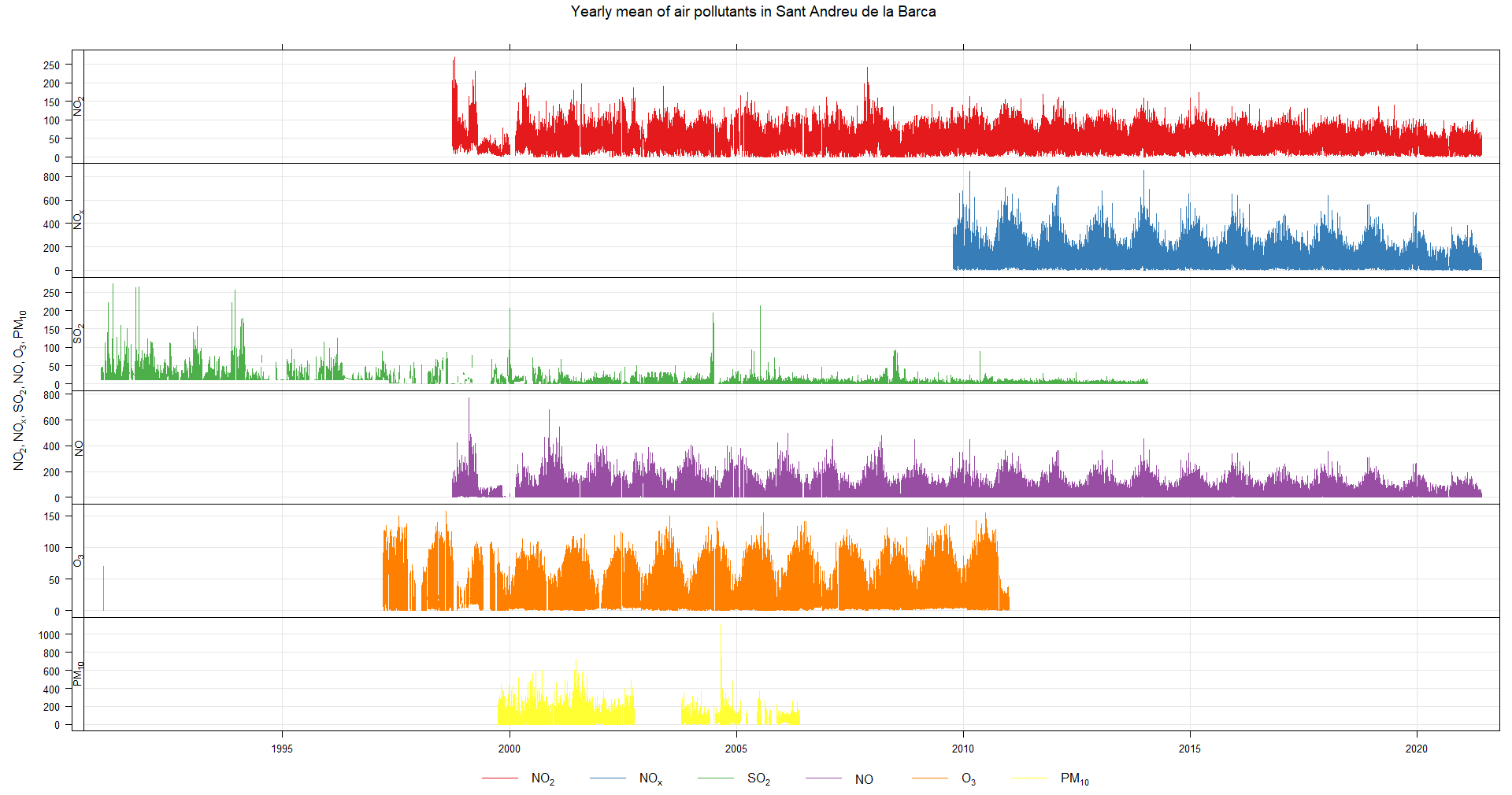
Time Plot 2:timePlot(selectByDate(city6), pollutant = c("NO2", "NOX", "SO2", "NO", "O3", "PM10"), y.relation = "free", main="Yearly mean of air pollutants in Sant Andreu de la Barca") |
 |
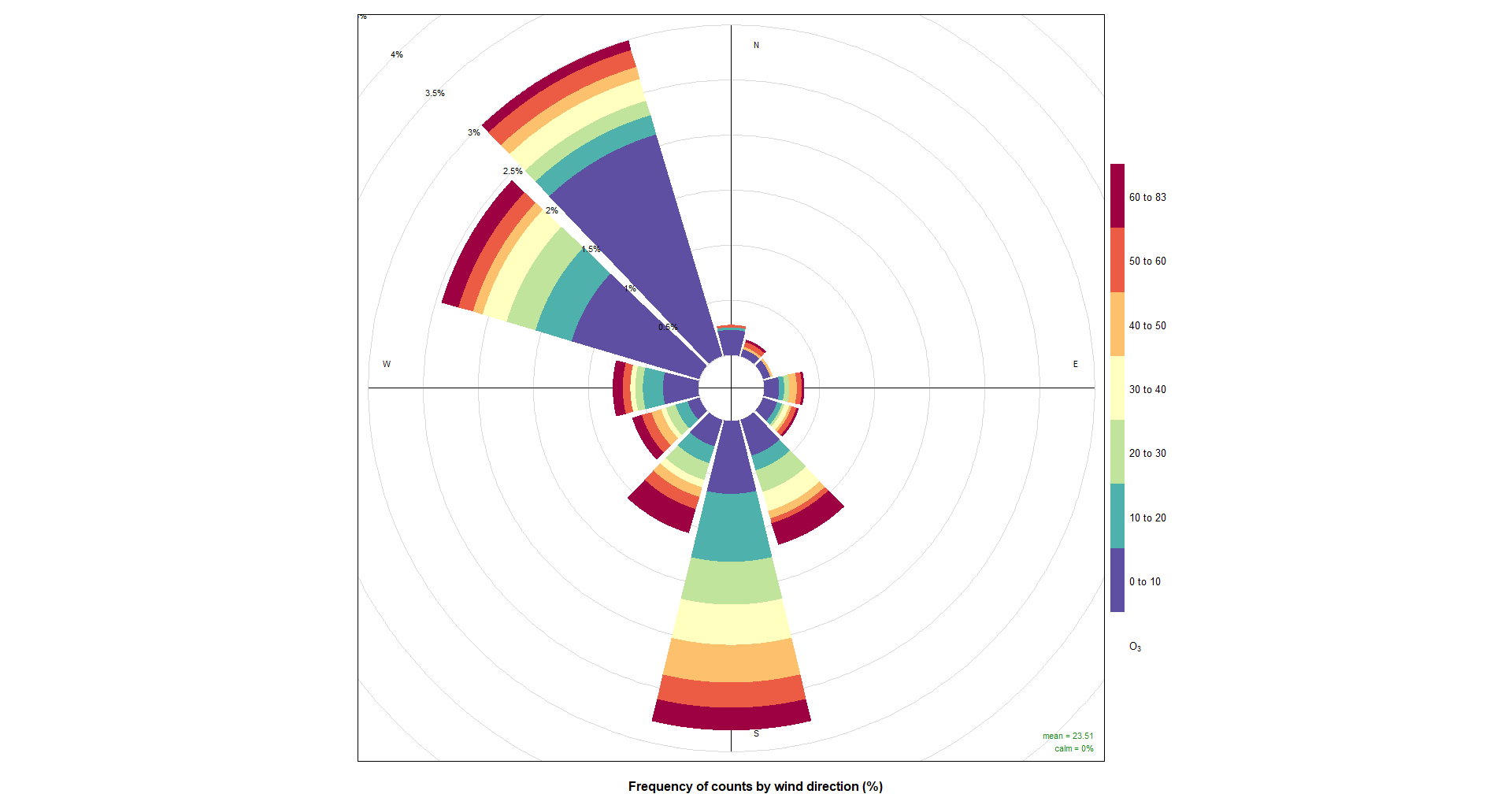
Pollution Rose:This code is a bit special so i will put It here, so you can follow all the steps: toDelete <- seq(2, nrow(wind3), 2) wind5<-wind3[ toDelete ,] cityall<-merge(city6, wind5, by = "date") pollutionRose(cityall, pollutant = "O3") |
 |
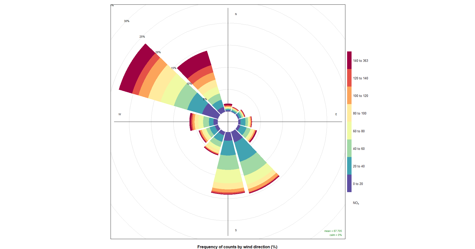
Pollution Rose 2:pollutionRose(cityall, pollutant = "NOX") |
 |
CONCLUSION:
With all the data that we have collected we could see If there are some values that exceed the legal limit of pollution and with the wind graphic (Pollution Rose) we could see where does the pollution come from.
The graphics are a good way to detect that high values of pollution and I think that this has been a good introduction into R language and a good way to learn basic code with RStudio as It has been very practic to work for the time with a large number of data.